

How To Construct A Covariance Matrix In Excel
This article is showing a geometric and intuitive explanation of the covariance matrix and the way it describes the shape of a data set. Nosotros will depict the geometric relationship of the covariance matrix with the use of linear transformations and eigendecomposition.
Introduction
Before we get started, nosotros shall take a quick look at the difference between covariance and variance. Variance measures the variation of a unmarried random variable (similar the superlative of a person in a population), whereas covariance is a measure of how much two random variables vary together (similar the height of a person and the weight of a person in a population). The formula for variance is given past
$$
\sigma^2_x = \frac{1}{north-1} \sum^{n}_{i=one}(x_i – \bar{10})^ii \\
$$
where \(n\) is the number of samples (e.g. the number of people) and \(\bar{x}\) is the mean of the random variable \(x\) (represented as a vector). The covariance \(\sigma(x, y)\) of two random variables \(x\) and \(y\) is given by
$$
\sigma(10, y) = \frac{1}{north-ane} \sum^{n}_{i=ane}{(x_i-\bar{x})(y_i-\bar{y})}
$$
with n samples. The variance \(\sigma_x^two\) of a random variable \(ten\) can be as well expressed as the covariance with itself by \(\sigma(x, 10)\).
Covariance Matrix
With the covariance we can calculate entries of the covariance matrix, which is a foursquare matrix given by \(C_{i,j} = \sigma(x_i, x_j)\) where \(C \in \mathbb{R}^{d \times d}\) and \(d\) describes the dimension or number of random variables of the information (e.g. the number of features like height, width, weight, …). Also the covariance matrix is symmetric since \(\sigma(x_i, x_j) = \sigma(x_j, x_i)\). The diagonal entries of the covariance matrix are the variances and the other entries are the covariances. For this reason, the covariance matrix is sometimes called the _variance-covariance matrix_. The calculation for the covariance matrix can be too expressed equally
$$
C = \frac{1}{n-1} \sum^{n}_{i=ane}{(X_i-\bar{Ten})(X_i-\bar{X})^T}
$$
where our information set is expressed by the matrix \(X \in \mathbb{R}^{n \times d}\). Following from this equation, the covariance matrix can exist computed for a data set with zero mean with \( C = \frac{XX^T}{northward-1}\) by using the semi-definite matrix \(20^T\).
In this article, we will focus on the two-dimensional example, only it tin exist hands generalized to more dimensional data. Post-obit from the previous equations the covariance matrix for two dimensions is given by
$$
C = \left( \brainstorm{array}{ccc}
\sigma(x, x) & \sigma(x, y) \\
\sigma(y, x) & \sigma(y, y) \end{array} \right)
$$
Nosotros want to show how linear transformations affect the information gear up and in result the covariance matrix. First nosotros will generate random points with mean values \(\bar{x}\), \(\bar{y}\) at the origin and unit of measurement variance \(\sigma^2_x = \sigma^2_y = one\) which is also called white noise and has the identity matrix as the covariance matrix.
import numpy every bit np import matplotlib.pyplot as plt %matplotlib inline plt.way.employ('ggplot') plt.rcParams['effigy.figsize'] = (12, 8) # Normal distributed x and y vector with mean 0 and standard difference 1 10 = np.random.normal(0, 1, 500) y = np.random.normal(0, 1, 500) X = np.vstack((10, y)).T plt.scatter(X[:, 0], X[:, ane]) plt.title('Generated Data') plt.centrality('equal'); 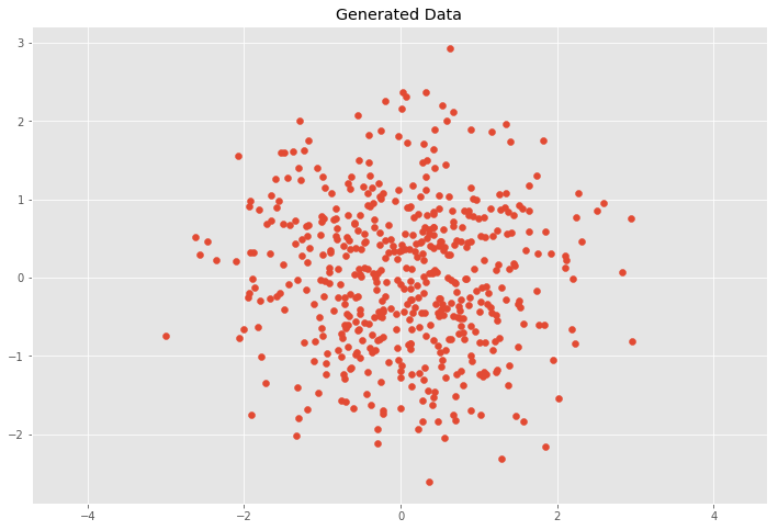
This case would mean that \(ten\) and \(y\) are independent (or uncorrelated) and the covariance matrix \(C\) is
$$
C = \left( \begin{array}{ccc}
\sigma_x^two & 0 \\
0 & \sigma_y^2 \stop{assortment} \right)
$$
We tin can bank check this past computing the covariance matrix
# Covariance def cov(x, y): xbar, ybar = x.mean(), y.mean() return np.sum((x - xbar)*(y - ybar))/(len(ten) - 1) # Covariance matrix def cov_mat(X): return np.array([[cov(X[0], X[0]), cov(X[0], X[1])], \ [cov(10[1], X[0]), cov(X[i], X[1])]]) # Calculate covariance matrix cov_mat(Ten.T) # (or with np.cov(10.T)) array([[ 1.008072 , -0.01495206], [-0.01495206, 0.92558318]])
Which approximatelly gives us our expected covariance matrix with variances \(\sigma_x^ii = \sigma_y^ii = 1\).
Linear Transformations of the Data Set
Next, we will look at how transformations bear upon our data and the covariance matrix \(C\). We will transform our information with the following scaling matrix.
$$
S = \left( \begin{array}{ccc}
s_x & 0 \\
0 & s_y \finish{array} \correct)
$$
where the transformation only scales the \(ten\) and \(y\) components by multiplying them by \(s_x\) and \(s_y\) respectively. What nosotros wait is that the covariance matrix \(C\) of our transformed data gear up will merely exist
$$
C = \left( \begin{array}{ccc}
(s_x\sigma_x)^2 & 0 \\
0 & (s_y\sigma_y)^2 \end{array} \right)
$$
which means that we tin extract the scaling matrix from our covariance matrix by calculating \(Due south = \sqrt{C}\) and the information is transformed by \(Y = SX\).
# Center the matrix at the origin 10 = X - np.mean(X, 0) # Scaling matrix sx, sy = 0.7, three.iv Scale = np.array([[sx, 0], [0, sy]]) # Employ scaling matrix to X Y = X.dot(Scale) plt.scatter(Y[:, 0], Y[:, one]) plt.title('Transformed Data') plt.axis('equal') # Summate covariance matrix cov_mat(Y.T) array([[ 0.50558298, -0.09532611], [-0.09532611, 10.43067155]]) 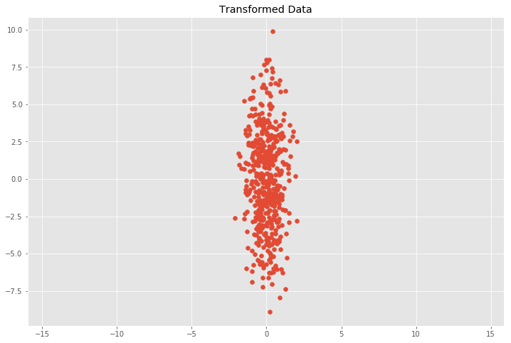
We can see that this does in fact approximately friction match our expectation with \(0.7^ii = 0.49\) and \(3.4^two = xi.56\) for \((s_x\sigma_x)^two\) and \((s_y\sigma_y)^2\). This relation holds when the data is scaled in \(x\) and \(y\) direction, merely it gets more involved for other linear transformations.
Now we volition apply a linear transformation in the form of a transformation matrix \(T\) to the data set which will be composed of a two dimensional rotation matrix \(R\) and the previous scaling matrix \(Southward\) equally follows
$$T = RS$$
where the rotation matrix \(R\) is given past
$$
R = \left( \brainstorm{assortment}{ccc}
cos(\theta) & -sin(\theta) \\
sin(\theta) & cos(\theta) \stop{array} \correct)
$$
where \(\theta\) is the rotation angle. The transformed data is and so calculated by \(Y = TX\) or \(Y = RSX\).
# Scaling matrix sx, sy = 0.7, 3.4 Scale = np.assortment([[sx, 0], [0, sy]]) # Rotation matrix theta = 0.77*np.pi c, s = np.cos(theta), np.sin(theta) Rot = np.array([[c, -s], [due south, c]]) # Transformation matrix T = Scale.dot(Rot) # Apply transformation matrix to X Y = Ten.dot(T) plt.besprinkle(Y[:, 0], Y[:, 1]) plt.title('Transformed Information') plt.centrality('equal'); # Calculate covariance matrix cov_mat(Y.T) array([[ 4.94072998, -4.93536067], [-four.93536067, 5.99552455]]) 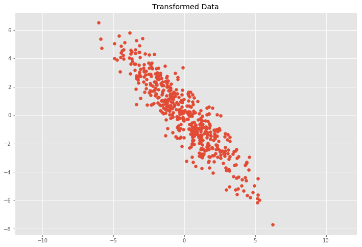
This leads to the question of how to decompose the covariance matrix \(C\) into a rotation matrix \(R\) and a scaling matrix \(Southward\).
Eigen Decomposition of the Covariance Matrix
Eigen Decomposition is 1 connection between a linear transformation and the covariance matrix. An eigenvector is a vector whose management remains unchanged when a linear transformation is practical to information technology. It tin can exist expressed every bit
$$ Av=\lambda five $$
where \(v\) is an eigenvector of \(A\) and \(\lambda\) is the corresponding eigenvalue. If we put all eigenvectors into the columns of a Matrix \(V\) and all eigenvalues as the entries of a diagonal matrix \(L\) nosotros can write for our covariance matrix \(C\) the following equation
$$ CV = VL $$
where the covariance matrix can be represented as
$$ C = VLV^{-1} $$
which can be too obtained by Atypical Value Decomposition. The eigenvectors are unit vectors representing the direction of the largest variance of the information, while the eigenvalues correspond the magnitude of this variance in the corresponding directions. This means \(5\) represents a rotation matrix and \(\sqrt{L}\) represents a scaling matrix. From this equation, we tin can correspond the covariance matrix \(C\) as
$$ C = RSSR^{-1} $$
where the rotation matrix \(R=V\) and the scaling matrix \(S=\sqrt{50}\). From the previous linear transformation \(T=RS\) we can derive
$$ C = RSSR^{-1} = TT^T $$
because \(T^T = (RS)^T=S^TR^T = SR^{-1}\) due to the properties \(R^{-ane}=R^T\) since \(R\) is orthogonal and \(S = S^T\) since \(S\) is a diagonal matrix. This enables the states to calculate the covariance matrix from a linear transformation. In order to calculate the linear transformation of the covariance matrix, i must summate the eigenvectors and eigenvectors from the covariance matrix \(C\). This can exist done by calculating
$$ T = V\sqrt{L} $$
where \(V\) is the previous matrix where the columns are the eigenvectors of \(C\) and \(50\) is the previous diagonal matrix consisting of the respective eigenvalues. The transformation matrix can be also computed by the Cholesky decomposition with \(Z = 50^{-1}(X-\bar{X})\) where \(L\) is the Cholesky factor of \(C = LL^T\).
We can see the basis vectors of the transformation matrix by showing each eigenvector \(5\) multiplied past \(\sigma = \sqrt{\lambda}\). Past multiplying \(\sigma\) with three nosotros comprehend approximately \(99.seven\%\) of the points according to the three sigma dominion if nosotros would depict an ellipse with the two ground vectors and count the points inside the ellipse.
C = cov_mat(Y.T) eVe, eVa = np.linalg.eig(C) plt.scatter(Y[:, 0], Y[:, 1]) for e, v in zip(eVe, eVa.T): plt.plot([0, 3*np.sqrt(e)*5[0]], [0, 3*np.sqrt(east)*v[ane]], 'k-', lw=two) plt.championship('Transformed Information') plt.centrality('equal'); 
Nosotros can now become from the covariance the transformation matrix \(T\) and we can utilize the inverse of \(T\) to remove correlation (whiten) the data.
C = cov_mat(Y.T) # Calculate eigenvalues eVa, eVe = np.linalg.eig(C) # Calculate transformation matrix from eigen decomposition R, S = eVe, np.diag(np.sqrt(eVa)) T = R.dot(Southward).T # Transform data with inverse transformation matrix T^-1 Z = Y.dot(np.linalg.inv(T)) plt.besprinkle(Z[:, 0], Z[:, i]) plt.title('Uncorrelated Data') plt.axis('equal'); # Covariance matrix of the uncorrelated data cov_mat(Z.T) array([[ 1.00000000e+00, -1.24594167e-16], [-ane.24594167e-xvi, ane.00000000e+00]]) 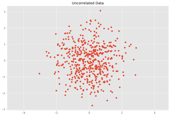
An interesting utilise of the covariance matrix is in the Mahalanobis altitude, which is used when measuring multivariate distances with covariance. It does that by calculating the uncorrelated altitude betwixt a point \(x\) to a multivariate normal distribution with the following formula
$$ D_M(ten) = \sqrt{(x – \mu)^TC^{-i}(10 – \mu))} $$
where \(\mu\) is the mean and \(C\) is the covariance of the multivariate normal distribution (the gear up of points causeless to be normal distributed). A derivation of the Mahalanobis distance with the apply of the Cholesky decomposition can exist found in this article.
Conclusion
In this article we saw the relationship of the covariance matrix with linear transformation which is an important building block for understanding and using PCA, SVD, the Bayes Classifier, the Mahalanobis distance and other topics in statistics and blueprint recognition. I found the covariance matrix to be a helpful cornerstone in the understanding of the many concepts and methods in blueprint recognition and statistics.
Many of the matrix identities tin can exist institute in The Matrix Cookbook. The relationship between SVD, PCA and the covariance matrix are elegantly shown in this question.

Source: https://datascienceplus.com/understanding-the-covariance-matrix/
Posted by: mcclearylonswellot.blogspot.com
0 Response to "How To Construct A Covariance Matrix In Excel"
Post a Comment